silico general demo

Introduction

import pandas as pd
import numpy as np
from numpy import random

import silico

Define a function that takes some parameters and returns a dict of information about the results:

def experiment_f(mean, sigma, seed):
    # All seeds should be initialized using a parameter for reproducibility
    random.seed(seed)
    # Return a dict with the results (must be pickleable)
    return {"value": random.normal(mean, sigma)}

Define the values for each of the parameters:

experiment = silico.Experiment(
    [
        ("mean", [1, 2, 4]),
        ("sigma", [1, 2, 3]),
        ("seed", list(range(20))),
    ],
    experiment_f,  # Function
    "experiment-demo",  # Folder where the results are stored
)

# If the definition of the experiment has changed, previous results can be deleted by running:
experiment.invalidate()

experiment.run_all()

To obtain a table with results:

df=experiment.get_results_df()
df

			_run_start	_elapsed_seconds	value
mean	sigma	seed
1	1	0	2023-03-23 01:20:53.154519	0.000054	2.764052
		1	2023-03-23 01:20:53.155430	0.000050	2.624345
		2	2023-03-23 01:20:53.156125	0.000030	0.583242
		3	2023-03-23 01:20:53.156363	0.000023	2.788628
		4	2023-03-23 01:20:53.156568	0.000021	1.050562
...	...	...	...	...	...
4	3	15	2023-03-23 01:20:53.187919	0.000010	3.063015
		16	2023-03-23 01:20:53.188014	0.000010	4.383846
		17	2023-03-23 01:20:53.188111	0.000009	4.828798
		18	2023-03-23 01:20:53.188217	0.000010	4.238285
		19	2023-03-23 01:20:53.188313	0.000010	4.663010

180 rows × 3 columns

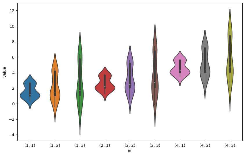
Plot and table generation

Some examples for figure and table generation follow

import matplotlib.pyplot as plt
import seaborn as sns

# Add an id field concatenating the two relevant levels of the index:
df["id"]=df.reset_index(["mean", "sigma"]).apply(lambda x: "(%s, %s)"%(x["mean"],x["sigma"]), axis=1).values

plt.figure(figsize=(10, 10 / 1.618))
sns.violinplot(
    data=df,
    x="id",
    y="value",
)
# plt.ylim(0.8, 1.1)
plt.show()

# Produce a table summarizing the mean values with its error
silico.df_agg_mean(df.drop(["_run_start", "id"], axis=1), ["mean", "sigma"])

		_elapsed_seconds	value
mean	sigma
1	1	0.000023 ± 0.000002	1.58 ± 0.19
	2	0.0000262 ± 0.0000014	2.2 ± 0.4
	3	0.0000219 ± 0.0000009	2.7 ± 0.6
2	1	0.000028 ± 0.000002	2.58 ± 0.19
	2	0.0000243 ± 0.0000014	3.2 ± 0.4
	3	0.000024 ± 0.000003	3.7 ± 0.6
4	1	0.0000156 ± 0.0000005	4.58 ± 0.19
	2	0.00000995 ± 0.00000009	5.2 ± 0.4
	3	0.00000975 ± 0.00000010	5.7 ± 0.6

Modifying task iteration order

Evaluation order is only important if you interfere with the run before it finishes (e.g, looking at intermediate results) or if you want to explore only a subset of the parameter space.

The default strategy follows an ordered array from inner to outer coordinates. The experiment definition could be manipulated to alter this, modifying the variable order or the values list.

# Check the chronological execution order in the previous example
df.sort_values("_run_start").index

MultiIndex([(1, 1,  0),
            (1, 1,  1),
            (1, 1,  2),
            (1, 1,  3),
            (1, 1,  4),
            (1, 1,  5),
            (1, 1,  6),
            (1, 1,  7),
            (1, 1,  8),
            (1, 1,  9),
            ...
            (4, 3, 10),
            (4, 3, 11),
            (4, 3, 12),
            (4, 3, 13),
            (4, 3, 14),
            (4, 3, 15),
            (4, 3, 16),
            (4, 3, 17),
            (4, 3, 18),
            (4, 3, 19)],
           names=['mean', 'sigma', 'seed'], length=180)

An alternative strategy can be used to explore the same grid in a different order by first picking the corners and the choosing always a point furthest away from already picked ones. This is called the urinal strategy, since this implements a protocol known by most men.

experiment_urinal = silico.Experiment(
    [
        ("mean", [1, 2, 4]),
        ("sigma", [1, 2, 3]),
        ("seed", list(range(20))),
    ],
    experiment_f,  # Function
    "experiment-demo-urinal",  # Folder where the results are stored
    strategy="urinal"
)

experiment_urinal.invalidate()
experiment_urinal.run_all()

# Now corners are first explored
experiment_urinal.get_results_df().sort_values("_run_start").index

MultiIndex([(1, 1,  0),
            (1, 1, 19),
            (1, 3,  0),
            (1, 3, 19),
            (4, 1,  0),
            (4, 1, 19),
            (4, 3,  0),
            (4, 3, 19),
            (2, 2,  9),
            (1, 1, 13),
            ...
            (4, 3,  5),
            (4, 3,  7),
            (4, 3,  8),
            (4, 3, 10),
            (4, 3, 11),
            (4, 3, 13),
            (4, 3, 14),
            (4, 3, 16),
            (4, 3, 17),
            (4, 3, 18)],
           names=['mean', 'sigma', 'seed'], length=180)

Finally, if you are interested on fixing a point and studying variations of only one variable, you might be interested in the star strategy, which first studies a special mid_point argument (default to the median for numerical data) and then explores each of the 1d subspaces.

experiment_star = silico.Experiment(
    [
        ("mean", [1, 2, 4]),
        ("sigma", [1, 2, 3]),
        ("seed", list(range(20))),
    ],
    experiment_f,
    "experiment-demo-star",
    strategy="star",
    mid_point={"mean":2,"sigma":2,"seed":10} # Default to the median for numerical data
)

experiment_star.invalidate()
experiment_star.run_all()

# Very few points (~sum of dims instead of product of dims)
experiment_star.get_results_df().sort_values("_run_start").index

MultiIndex([(2, 2, 10),
            (1, 2, 10),
            (4, 2, 10),
            (2, 1, 10),
            (2, 3, 10),
            (2, 2,  0),
            (2, 2,  1),
            (2, 2,  2),
            (2, 2,  3),
            (2, 2,  4),
            (2, 2,  5),
            (2, 2,  6),
            (2, 2,  7),
            (2, 2,  8),
            (2, 2,  9),
            (2, 2, 11),
            (2, 2, 12),
            (2, 2, 13),
            (2, 2, 14),
            (2, 2, 15),
            (2, 2, 16),
            (2, 2, 17),
            (2, 2, 18),
            (2, 2, 19)],
           names=['mean', 'sigma', 'seed'])

You can also run sequentially multiple Experiment instances with the same function in the same folder to achieve other strategies.

A SubExperiment class is also available to restrict some of the parameters.

list(silico.SubExperiment(experiment, {"mean":3, "seed":5}).iter_values())

[{'sigma': 1}, {'sigma': 2}, {'sigma': 3}]

Loading from a module and execution modes

The best practice is to define the experiment in a module

import demo

In this example we include a delay in the function to understand the execution modes

# Check for demo purpose
import inspect
print(inspect.getsource(demo.experiment.f))

def experiment_f(mean, sigma, seed):
    # All seeds should be initialized using a parameter for reproducibility
    random.seed(seed)
    # Delay for test purpose
    sleep(mean/100)
    # Return a dict with the results (must be pickleable)
    return {"value": random.normal(mean, sigma)}

Sequential execution

The default mode is sequential execution (all trials are executed one by one).

Advantages:

• All memory/cpu resources available

• Execution time is not affected by other processes

Disadvantages:

• Longest execution time

demo.experiment.invalidate()

%%time
demo.experiment.run_all()

CPU times: user 210 ms, sys: 30.6 ms, total: 240 ms
Wall time: 4.42 s

sum(demo.experiment.get_results_df()["_elapsed_seconds"])

4.246137000000002

Multithreading execution

In multithreading execution a pool of threads run the trials.

Advantages:

• If n threads are used and the trial uses only one thread, you can expect a factor of n speed-up, assumming your resources are not exhausted.

• Does not require additional libraries.

Disadvantages:

• Memory consumption increases

• Concurrent execution might affect computation time

• Only one machine can be used still.

demo.experiment.invalidate()

In this example we use 4 threads for a ~4x speed-up:

%%time
demo.experiment.run_all(method="multithreading", threads=4)

CPU times: user 73.2 ms, sys: 60.1 ms, total: 133 ms
Wall time: 1.17 s

However, elapsed time is independent for each trial, so the total is approximately the same

sum(demo.experiment.get_results_df()["_elapsed_seconds"])

4.24141